Pitch Detection and Auto-Calibration
The three-metric detector caught most noise. These two additions handled the rest.
The three-metric detector from the previous post — energy, zero-crossing rate, spectral centroid — solved the keyboard clicking problem and most transient noise. Two issues remained. First, some sounds with speech-like frequency characteristics still got through. Second, the thresholds were hardcoded, which meant the detector worked in one acoustic environment and failed in another.
Pitch detection addressed the first problem. Auto-calibration addressed the second.
Why pitch matters
Human speech is quasi-periodic. When you produce a vowel sound, your vocal cords vibrate at a fundamental frequency — typically between 80 Hz for a low male voice and 300 Hz for a high female voice. This periodicity is absent from most environmental noise. Keyboard clicks, traffic, HVAC systems, conversations in adjacent rooms — none of these have the regular periodic structure of a single human voice.
The zero-crossing rate and spectral centroid already capture some of this distinction indirectly. But they are aggregate statistics. A sound with moderate ZCR and moderate spectral centroid could be voiced speech, or it could be a mix of noise sources that average out to speech-like values. Pitch detection asks a more direct question: is there a repeating pattern in this signal?
Autocorrelation
The standard approach to pitch detection in the time domain is autocorrelation. You correlate the signal with a delayed copy of itself, sweep across a range of delay values, and look for a peak. If the signal is periodic, the autocorrelation will peak at a lag equal to the period.
int minLag = sampleRate / 400; // 400 Hz upper bound
int maxLag = sampleRate / 80;  // 80 Hz lower bound
double[] autocorr = new double[maxLag + 1];

for (int lag = 0; lag <= maxLag; lag++) {
  for (int i = 0; i < buffer.length - lag; i++) {
    autocorr[lag] += buffer[i] * buffer[i + lag];
  }
}
At 8000 Hz sample rate, the search range is lag 20 (400 Hz) to lag 100 (80 Hz). For each lag value, the inner loop multiplies each sample by the sample that many positions ahead and sums the results. If the signal repeats at that period, the products are consistently positive — the signal aligns with itself. If there is no periodicity, the products cancel out.
Interactive visualization showing autocorrelation-based pitch detection comparing voiced speech with a clear peak versus keyboard click noise with no clear peak
Voiced speech — "ah"
Autocorrelation shows a clear periodic peak
Keyboard click
No periodic structure — autocorrelation decays monotonically
The peak lag gives the pitch period. The pitch frequency is sampleRate / peakLag. But the presence of a peak is more useful than the frequency itself. What I needed was not "the speaker's voice is at 151 Hz" but "there is periodic structure in this signal."
Pitch strength over pitch value
The first implementation simply checked whether the autocorrelation at the peak lag was positive. This was unreliable. A barely positive value in a noisy signal means nothing — the autocorrelation of random noise will have small positive and negative values scattered across all lags.
The fix was to normalize the peak against the autocorrelation at lag zero, which represents the total energy of the signal:
double pitchStrength = (autocorr[0] != 0)
    ? autocorr[peakLag] / autocorr[0]
    : 0;

double pitch = (pitchStrength > MIN_PITCH_STRENGTH)
    ? sampleRate / (double) peakLag
    : 0;
A pitchStrength of 1.0 means the signal is perfectly periodic. A value of 0.0 means no periodicity. In practice, clean voiced speech produces pitch strength in the 0.5 to 0.9 range. Keyboard clicks are typically below 0.15. I set MIN_PITCH_STRENGTH to 0.3 after testing with several voice types and noise conditions.
This made pitch strength a fourth metric available to the voice detection logic, though I used it more conservatively than the other three. The primary decision still relied on energy, ZCR, and spectral centroid. Pitch strength served as a confirming signal — a way to increase confidence in edge cases where the other metrics were ambiguous.
The cost of autocorrelation
Pitch detection is not free. The nested loop — for each of roughly 80 lag values, iterate across the entire buffer — is O(N × L) where N is the buffer size and L is the lag range. At 160 samples per 20ms chunk and 80 lag values, that is 12,800 multiply-and-accumulate operations per chunk, eight thousand times per second.
On a modern CPU this is negligible. But in a system that processes audio from potentially many concurrent calls, it adds up. I kept the implementation simple rather than optimizing with FFT-based autocorrelation, because the bottleneck was never computation — it was the network latency of the WebSocket pipeline and the transcription API calls. If the system needed to scale to thousands of concurrent streams, the FFT approach would be worth revisiting.
Auto-calibration
The three-metric detector and the pitch addition solved the feature extraction problem. The threshold problem remained. Every threshold — energy, ZCR, spectral centroid, pitch strength — depended on the acoustic environment. A quiet home office and a busy street produce fundamentally different ambient noise profiles. Hardcoded thresholds meant choosing between sensitivity and specificity.
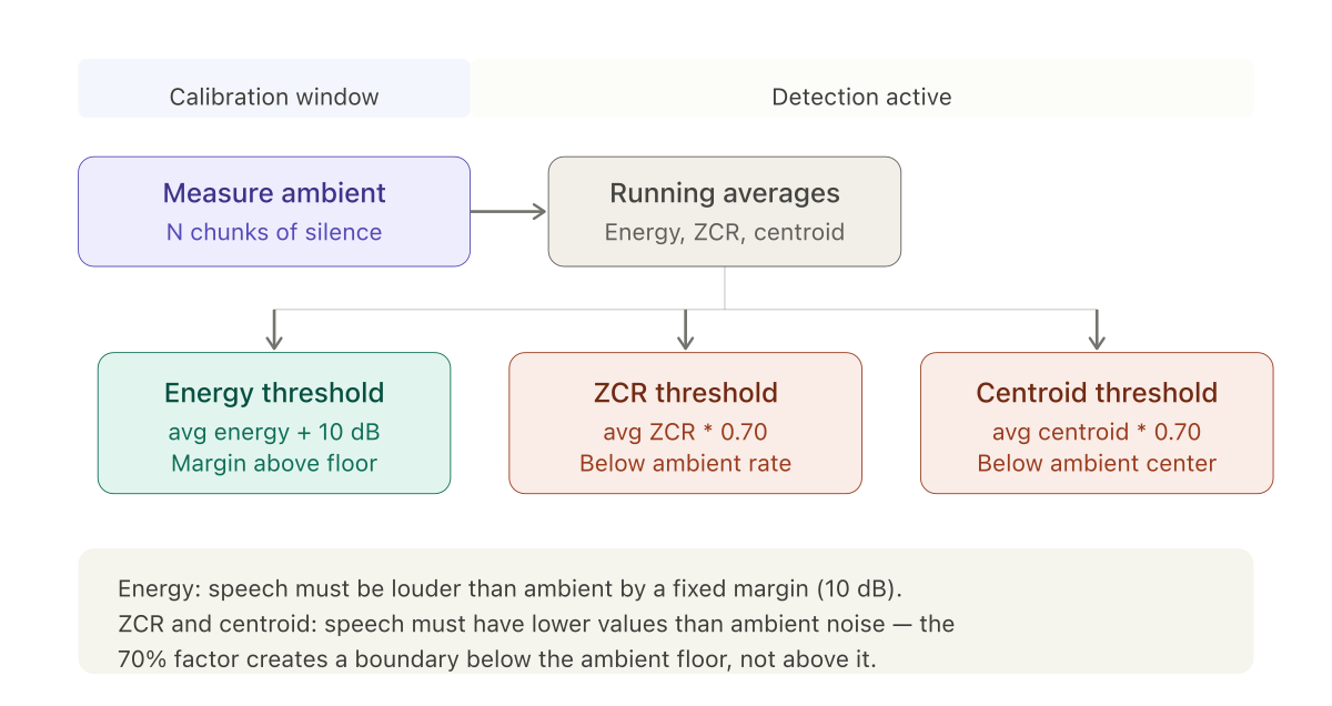
The solution was a calibration window at the start of each call. For the first N chunks of audio — before any speech is expected — the system measures the ambient environment and derives thresholds from what it observes.
The calibration state accumulates running totals:
calibrationCount++;
totalCalibrationEnergy += metrics.energy();
totalCalibrationZcr += metrics.zcr();
totalCalibrationSpectralCentroid += metrics.spectralCentroid();
When the calibration window closes, thresholds are derived from the averages:
double avgEnergy   = totalCalibrationEnergy   / calibrationCount;
double avgZcr      = totalCalibrationZcr      / calibrationCount;
double avgCentroid = totalCalibrationSpectralCentroid / calibrationCount;

double energyThreshold           = avgEnergy   + 10;   // +10 dB above ambient
double zcrThreshold              = avgZcr      * 0.70; // 70% of ambient ZCR
double spectralCentroidThreshold = avgCentroid * 0.70;
The asymmetry in threshold direction
The energy threshold sits above the ambient average. This is intuitive — speech must be louder than the background.
The ZCR and spectral centroid thresholds sit below the ambient average. This is counterintuitive until you remember what these metrics measure. In the isVoice logic, speech must have ZCR and centroid values lower than the threshold. The threshold is set at 70% of the ambient level, meaning speech must have lower ZCR and lower spectral centroid than the ambient noise floor.
This works because ambient noise — HVAC hum, street sounds, room tone — tends to have a scattered, broadband character. Its ZCR is moderate to high. Its spectral centroid is spread. Human speech, with its concentrated frequency energy and quasi-periodic structure, sits below these ambient values.
The 10 dB energy margin and the 0.70 multiplier were tuned empirically. Values between 0.60 and 0.80 for the frequency metrics all produced acceptable results. Threshold tuning is mostly about finding a stable midpoint.
The zero-calibration case
Not all calls start with silence. Sometimes the caller begins speaking immediately, or there is music playing before the conversation starts. The system needed a fallback for cases where the calibration window captured speech or non-ambient audio.
The fallback was a default threshold from configuration: defaultSilenceThreshold at -30 dBFS. If calibration is set to zero duration — effectively disabled — the system uses this default and the 0.70 multipliers against assumed ambient values. This is less accurate than environment-specific calibration, but it is better than nothing. In practice, the calibration window could be set as short as 500ms — 25 chunks at 20ms each — which was fast enough that most callers had not started speaking yet.
The state machine
With calibration, pitch detection, and the three-metric decision logic in place, the VAD operated as a simple state machine. It started in a calibration state, collecting ambient measurements. After the calibration window closed, it transitioned to a listening state, evaluating each chunk against the calibrated thresholds. When voice was detected, it entered a recording state, accumulating audio chunks. When silence returned — no voice detected for a configurable timeout period — it finalized the speech segment and emitted it for processing.
The voiceLastDetectedAt timestamp tracked when speech was last identified. The silence timeout compared the current time against this timestamp. This allowed for brief pauses within a sentence — normal speech contains short silences between words and phrases — without prematurely ending the segment. A timeout of one second accommodated natural pauses while keeping response latency acceptable.
This was the complete detection system. Everything after this — the WebSocket integration, the speech segment packaging, the handoff to transcription — was pipeline work rather than signal processing. The next post covers that pipeline: how the Twilio media stream protocol works, how audio chunks are accumulated into speech segments with correct byte alignment, and how the whole system fits into a Spring Boot WebSocket handler.